Exercises 22 | Surface Laplacian

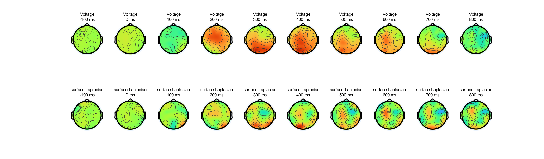
  1. Based on the topographical maps of ERPs in figure 22.6 (plate 12) , select one electrode whose activity you think might look similar before and after computing the surface Laplacian, and one electrode whose activity you think might look different before and after the surface Laplacian.

    (1) look similar before and after computing the surface Laplacian: FC1

    (2) look different before and after the surface Laplacian: PO8

    Figure22.6

  2. Perform a time-frequency decomposition of the data from those two electrodes both before and after computing the surface Laplacian (that is, compute the surface Laplacian on the raw data before applying a time-frequency decomposition). Compute both power (decibels normalized using a baseline period of your choice) and ITPC.

  3. Plot the results using the same color scaling for before and after the surface Laplacian.

%% 获得Surface Laplacian处理前后的数据
load sampleEEGdata.mat
% extract XYZ coordinates from EEG structure
X = [EEG.chanlocs.X];
Y = [EEG.chanlocs.Y];
Z = [EEG.chanlocs.Z];
% compute surface laplacian
lap_data = laplacian_perrinX(EEG.data,X,Y,Z);

%% 计算Power
electrode = ["FC1", "PO8" ,"FC4"];
electrodeidx = zeros(size(electrode));
for i = 1:length(electrode)
electrodeidx(i) = find(strcmpi({EEG.chanlocs.labels},electrode(i)));
end
frequencies = logspace(log10(2),log10(40),30);
%% calculate power

% perform filter-Hilber
% parameters of filter

freqspread = linspace(0.8,6,length(frequencies)); % Hz +/- the center frequency
transwid = 0.1;
nyquist = repmat(EEG.srate/2, size(frequencies));

% construct filter kernels
ffrequencies = [ ones(length(frequencies),1) (1-transwid).*(frequencies-freqspread)' (frequencies-freqspread)' (frequencies+freqspread)' (1+transwid).*(frequencies+freqspread)' nyquist' ]./nyquist(1);
idealresponse = [ 0 0 1 1 0 0 ];
filter_result = zeros(length(electrode),length(frequencies),3*EEG.pnts,EEG.trials);
filter_result_lap = zeros(length(electrode),length(frequencies),3*EEG.pnts,EEG.trials);

for electrodei = 1:length(electrode)
data2filter = [flipud(squeeze(EEG.data(electrodeidx(electrodei),:,:))); squeeze(EEG.data(electrodeidx(electrodei),:,:)); flipud(squeeze(EEG.data(electrodeidx(electrodei),:,:)))];
data2filter_lap= [flipud(squeeze(lap_data(electrodeidx(electrodei),:,:))); squeeze(lap_data(electrodeidx(electrodei),:,:)); flipud(squeeze(lap_data(electrodeidx(electrodei),:,:)))];
for fi = 1:length(frequencies)
filterweights = firls(100,ffrequencies(fi,:),idealresponse);
filter_result(electrodei,fi,:,:) = hilbert(filtfilt(filterweights,1,data2filter));
filter_result_lap(electrodei,fi,:,:) = hilbert(filtfilt(filterweights,1,data2filter_lap));
end
end
filter_result = filter_result(:,:,end/3+1:end*2/3,:);
filter_result_lap = filter_result_lap(:,:,end/3+1:end*2/3,:);
power_result = squeeze(mean(abs(filter_result).^2,4));
power_result_lap = squeeze(mean(abs(filter_result_lap).^2,4));
% define baseline period
baselinetime = [-500 -200 ]; % in ms

% convert baseline window time to indices
[~,baselineidx(1)]=min(abs(EEG.times-baselinetime(1)));
[~,baselineidx(2)]=min(abs(EEG.times-baselinetime(2)));

% dB-correct
baseline_power = mean(power_result(:,:,baselineidx(1):baselineidx(2)),3);
baseline_power_lap = mean(power_result_lap(:,:,baselineidx(1):baselineidx(2)),3);
power_dbconverted = 10*log10( bsxfun(@rdivide,power_result,baseline_power));
power_dbconverted_lap = 10*log10( bsxfun(@rdivide,power_result_lap,baseline_power_lap));


%% calculate ITPC
ITPC = abs(mean(exp(1i*angle(filter_result)),4));
ITPC_lap = abs(mean(exp(1i*angle(filter_result_lap)),4));

%% plot
time2plot = [-300, 1000];
time2plotidx = zeros(size(time2plot));
for i = 1:2
[~,time2plotidx(i)] = min(abs(EEG.times-time2plot(i)));
end


for electrodei = 1:length(electrode)
figure(electrodei)
subplot(2,2,1)
contourf(EEG.times(time2plotidx(1):time2plotidx(2)),frequencies,squeeze(power_dbconverted(electrodei,:,time2plotidx(1):time2plotidx(2))),30,'linecolor','none');
colormap jet
set(gca,'clim',[-3 3])
title({'Before Laplacian', ['Power from ' num2str(electrode(electrodei))]})

subplot(2,2,2)
contourf(EEG.times(time2plotidx(1):time2plotidx(2)),frequencies,squeeze(ITPC(electrodei,:,time2plotidx(1):time2plotidx(2))),30,'linecolor','none');
colormap jet
set(gca,'clim',[0 0.3])
title({'Before Laplacian', ['ITPC from ' num2str(electrode(electrodei))]})

subplot(2,2,3)
contourf(EEG.times(time2plotidx(1):time2plotidx(2)),frequencies,squeeze(power_dbconverted_lap(electrodei,:,time2plotidx(1):time2plotidx(2))),30,'linecolor','none');
colormap jet
set(gca,'clim',[-3 3])
title({'After Laplacian', ['Power from ' num2str(electrode(electrodei))]})

subplot(2,2,4)
contourf(EEG.times(time2plotidx(1):time2plotidx(2)),frequencies,squeeze(ITPC_lap(electrodei,:,time2plotidx(1):time2plotidx(2))),30,'linecolor','none');
colormap jet
set(gca,'clim',[0 0.3])
title({'After Laplacian', ['ITPC from ' num2str(electrode(electrodei))]})
end

Ex_22(1)

Ex_22(2)

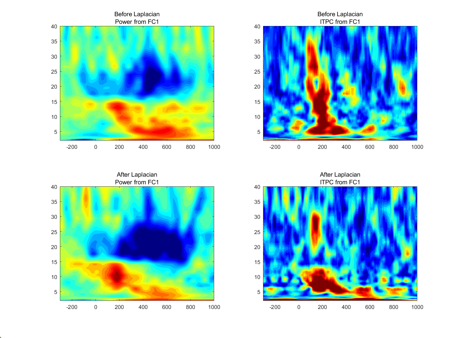
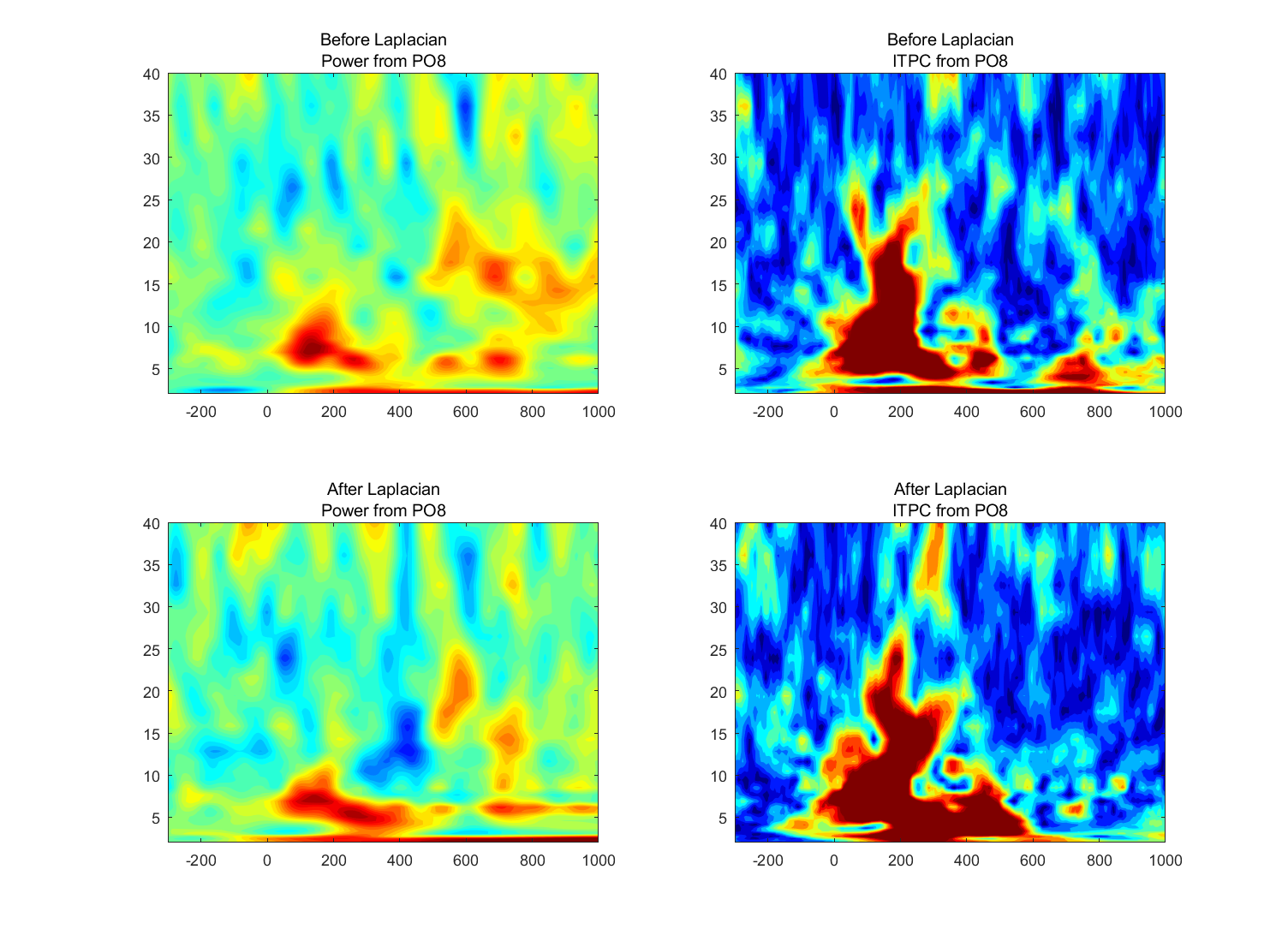
  1. Are there any salient differences in the time-frequency power or ITPC results before versus after application of the surface Laplacian, and do the differences depend on the frequency? How would you interpret similarities and differences at different frequency bands?
  • There are differences and the differences depend on the frequency, like the power from PC1 at 10 Hz and from PO8 at 15 Hz.

Exercises 23 | Principal Components Analysis (PCA)

  1. Perform PCA on broadband data using two time windows, one before and one after trial onset (e.g., – 500 to 0 ms and 100 to 600 ms).

  2. Plot topographical maps and time courses of the first four components. To construct the PCA time courses, multiply the PCA weights defined by the pre- and posttrial time windows with the electrode time courses from the entire trial. Do you notice any differences in the topographical maps or time courses from before versus after stimulus onset? How would you interpret differences and/or similarities?

  3. Repeat this exercise but after bandpass filtering in two different frequency bands. Make sure there are no edge artifacts in the pretrial time window (consider using reflection, if necessary, as described in figure 7.3). Justify your decision of frequency bands and time window width(s). Comment on any qualitative similarities and differences you observe between frequency bands and time windows and similarities and differences between the frequencyband-specific and broadband signal from the results obtained in the previous exercise.