Chap.25 Introduction to the Various Connectivity Analyses

Connectivity：指在同一时刻下考虑多个信号的分析。
需区分的概念：
- functional connectivity：linear or nonlinear covariation between fluctuations in activity recorded from distinct neural networks. 更接近于相关性（correlation）
- effective connectivity：a causal influence of activity in one neural network over activity in another neural network. 更接近于因果关系（causation）
两个电极之间的连接性（connectivity）可以反映不同大脑区域之间的真实连接，也可能是由于这两个电极测量了来自同一脑源的活动。

Chap.26 Phase-Based Connectivity

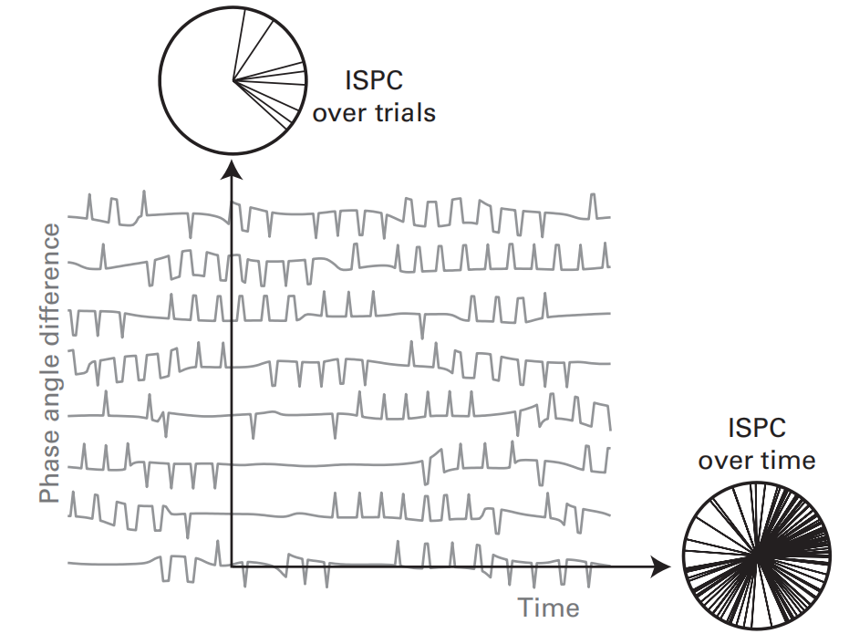
ISPC (Intersite phase clustering)

ISPC是一种用以描述基于相位的功能连接的方法，与ITPC相似，但计算的是两电极之间随时间或试次变化的相位角差的平均值

$ISPC_f=|n^{-1}\sum^n_{t=1}e^{i(\phi_{xt}-\phi_{yt})}|$

其中 n 是时间点数目或试次数目，$\phi_x$ 和 $\phi_{y}$ 是电极 x 和 y 在频率f下的相角，t是时间点或试次。

ISPC反映的不是两电极相位差的大小，而是相位差随时间或试次的一致性
ISPC是无向的（A→B的ISPC和B→A的相同）

ISPC-time and ISPC-trial

通过上面的公式，我们可以得到的是在一个时间窗口内一个试次的ISPC，如果有多个试次，而且我们想要得到ISPC随时间/试次的变化，可以采用如下方法：

ISPC-time：设置一个滑动的小时间窗，计算单个试次在每个时间窗下的ISPC（类似于short-time FFT），得到多个试次下的ISPC随时间的变化，最后再进行试次平均，得到ISPC在不同时刻下的值。小时间窗的长度选取规则类似于wavelet中the number of cycles的选取。
ISPC-trials：关注某一时间点下不同试次的相位差大小。ISPC-trial所反映是在不同的试次下，两电极间的相位差是否能保持一致，其值越大，说明相位差在不同试次下越能保持一致。
- 对试次的数目比较敏感，试次数目需要足够多，才能获得稳定的结果
- 如果在不同实验条件下的试次不同，可以考虑使用 weighted ISPC-trials (wISPC-trials)，其原理与 wITPC 相近。
计算时的区别：
- ISPC-time：先在滑动时间窗内时间平均，最后试次平均
- ISPC-trial：在不同时间点下进行试次平均

Matlab代码实现：

% 对于频率，通常采用对数分布
freqs2use  = logspace(log10(4),log10(30),15); % 4-30 Hz in 15 steps
% 非频率值，可以采用线性分布，timewindow的宽度是下面取值的两倍
timewindow = linspace(1.5,3,length(freqs2use)); % number of cycles on either end of the center point (1.5 means a total of 3 cycles))

ISPC-time (ispc) 和 ISPC-trial (ps) 的计算：

for fi=1:length(freqs2use)
    % phase angle differences（维度为time×trials）
    phase_diffs = phase_sig1-phase_sig2;
    
    % compute ISPC over trials（trial平均，时间没有平均，所以ps的是"频率×时间"的矩阵）
    ps(fi,:) = abs(mean(exp(1i*phase_diffs(times2saveidx,:)),2));
    
    % 计算每一个时间点（timewindow中点）下的ISPC
    for ti=1:length(times2save)
        
        % compute phase synchronization（ISPC-time，每个时间窗可计算出一个值，1×trial）
        phasesynch = abs(mean(exp(1i*phase_diffs(times2saveidx(ti)-time_window_idx:times2saveidx(ti)+time_window_idx,:)),1));
        
        % average over trials（trial平均）
        ispc(fi,ti) = mean(phasesynch);
    end
end % end frequency loop

最后可以让每个时间点减去baseline时间内的ISPC平均值，突出任务相关影响：

% ISPC-time
contourf(times2save,freqs2use,ispc-repmat(mean(ispc(:,baselineidx(1):baselineidx(2)),2),1,size(ispc,2)),20,'linecolor','none')

% ISPC-trial
contourf(times2save,freqs2use,bsxfun(@minus,ps,mean(ps(:,baselineidx(1):baselineidx(2)),2)),20,'linecolor','none')

Spectral Coherence (Magnitude-Squared Coherence) | 波谱相干

波谱相干可以理解为是把信号功率作为权重的加权ISPC

公式

常见的波谱相干公式：

$Coher_{xy}=\left| \frac{S_{xy}}{S_{xx}S_{yy}}\right|$

$S_{xy}$ 是电极x和y处的互功率谱密度，$S_{xx}$ 和 $S_{yy}$ 是电极x和y处的自功率谱密度。上式中的分子有时会平方，从而和分母的量级相配合。

为便于理解，可以将波谱相干公式写成下面的形式：

$C_{xy}=\left| n^{-1}\sum^n_{t=1}\lvert m_{tx}m_{ty}\rvert e^{i\phi_{txy}}\right|^{2}$

$m_x$和$m_y$是解析信号（没有负频率分量的复值函数）X和Y的功率大小（magnitudes），$\phi_{xy}$是电极X和Y之间的相位角差，t指trial或时间点。

可以发现使用这一公式计算出的$C_{xy}$值会随着功率大小改变，而功率又会随频率、时间、任务等改变，所以可以将这一公式进行归一化，得到如下波谱相干公式：

$Coher_{xy}=\frac{C_{xy}}{\left(n^{-1}\sum^n_{t=1}|m_{tx}|^2\right)\left(n^{-1}\sum^n_{t=1}|m_{ty}|^2\right)}$

由这种方法得到的波谱相干性大小将介于0和1之间，1代表完全相干，0代表完全独立。

Matlab代码实现

计算自功率谱大小时，使用信号乘以其共轭的方法 sig1.*conj(sig1)，耗时比直接平方(sig1).^2更短
计算互功率谱$S_{xy}$时，使用信号1乘以信号2的共轭的方法sig1.*conj(sig2)，耗时比欧拉公式abs(sig1).*abs(sig2).*exp(1i*(angle(sig1)-angle(sig2)))更短

% select channels
channel1 = 'fz';
channel2 = 'o1';

% wavelet and FFT parameters
time          = -1:1/EEG.srate:1;
half_wavelet  = (length(time)-1)/2;
n_wavelet     = length(time);
n_data        = EEG.pnts*EEG.trials;       
n_convolution = n_wavelet+n_data-1;

chanidx    = zeros(1,2); % always initialize!
chanidx(1) = find(strcmpi(channel1,{EEG.chanlocs.labels}));
chanidx(2) = find(strcmpi(channel2,{EEG.chanlocs.labels}));

% data FFTs （把一个电极里所有trial的数据排列成一个行向量，减少计算的次数）
data_fft1 = fft(reshape(EEG.data(chanidx(1),:,:),1,n_data),n_convolution);
data_fft2 = fft(reshape(EEG.data(chanidx(2),:,:),1,n_data),n_convolution);


% initialize
spectcoher = zeros(length(freqs2use),length(times2save));

for fi=1:length(freqs2use)
    
    % create wavelet and take FFT
    s = num_cycles(fi)/(2*pi*freqs2use(fi));
    wavelet_fft = fft( exp(2*1i*pi*freqs2use(fi).*time) .* exp(-time.^2./(2*(s^2))) ,n_convolution);
    
    % phase angles from channel 1 via convolution
    convolution_result_fft = ifft(wavelet_fft.*data_fft1,n_convolution);
    convolution_result_fft = convolution_result_fft(half_wavelet+1:end-half_wavelet);
    % 把原来排成一行的结果变回 electrodes×trials
    sig1 = reshape(convolution_result_fft,EEG.pnts,EEG.trials);
    
    % phase angles from channel 2 via convolution
    convolution_result_fft = ifft(wavelet_fft.*data_fft2,n_convolution);
    convolution_result_fft = convolution_result_fft(half_wavelet+1:end-half_wavelet);
    % 把原来排成一行的结果变回 electrodes×trials
    sig2 = reshape(convolution_result_fft,EEG.pnts,EEG.trials);
    
    % compute power and cross-spectral power
    % 自功率谱
    spec1 = mean(sig1.*conj(sig1),2);
    spec2 = mean(sig2.*conj(sig2),2);
    % 交叉功率谱的平方
    specX = abs(mean(sig1.*conj(sig2),2)).^2;
    
    % alternative notation for the same procedure, using the Euler-like expression: Me^ik
    %spec1 = mean(abs(sig1).^2,2);
    %spec2 = mean(abs(sig2).^2,2);
    %specX = abs(mean( abs(sig1).*abs(sig2) .* exp(1i*(angle(sig1)-angle(sig2))) ,2)).^2;

    % 计算Coherence。compute spectral coherence, using only requested time points
    spectcoher(fi,:) = specX(times2saveidx)./(spec1(times2saveidx).*spec2(times2saveidx));
    
    % yet another equivalent notation, just FYI
    %spec1 = sum(sig1.*conj(sig1),2);
    %spec2 = sum(sig2.*conj(sig2),2);
    %specX = sum(sig1.*conj(sig2),2);
    %spectcoher(fi,:) = abs(specX(times2saveidx)./sqrt(spec1(times2saveidx).*spec2(times2saveidx))).^2;
   
end

最终的结果可以减去baseline时间段的coherence：

contourf(times2save,freqs2use,spectcoher-repmat(mean(spectcoher(:,baselineidx(1):baselineidx(2)),2),1,size(spectcoher,2)),20,'linecolor','none')

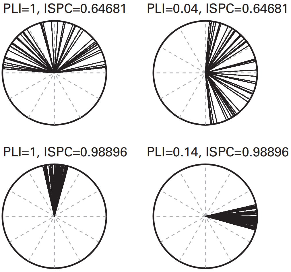
Phase Lag-Based Measures

spurious connectivity results that are caused by two electrodes measuring activity from the same source will have phase lags of zero or $\pi$ ( $\pi$ if the electrodes are on opposite sides of the dipole). 由体积传导（同源）引起的相位差通常为0或$\pi$。

Imaginary Coherence

Imaginary coherence uses almost the same equation as that for spectual coherence, except the imaginary part of te spectual coherence is taken before the magnitude.

% imaginary coherence
    spec1 = sum(sig1.*conj(sig1),2); %imaginart
    spec2 = sum(sig2.*conj(sig2),2);
    specX = sum(sig1.*conj(sig2),2);
    spectcoher(fi,:) = abs(imag(specX(times2saveidx)./sqrt(spec1(times2saveidx).*spec2(times2saveidx))));

Phase-Lag Index（PLI）

根据上面的结论，我们可以有一个感性的认识：由体积传导引起的相位差通常分布在极坐标的0或$\pi$附近（关于实轴对称，指向左右），而不含体积传导的相位差将会分布在虚轴的正半轴或负半轴附近（关于虚轴对称，指向上下）。

The Phase-lag index（PLI）就通过计算互功率谱密度的虚部符号平均值，来定量地描述相位信号受体积传导效应影响的大小：

$PLI_{xy}=\left| n^{-1}\sum^n_{i=1}sgn(imag(S_{xyt})) \right|$

The weighted phase-lag index（wPLI）通过添加一个权重，使得离虚轴越近（虚部越大）的互功率谱密度值对PLI的贡献更大：

$PLI_{xy}=\frac{n^{-1} \sum^n_{i=1}\left|imag(S_{xyt}) \right|sgn(imag(S_{xyt}))}{n^{-1} \sum^n_{i=1}\left|imag(S_{xyt}) \right|}$

The phase-slope index

略

Mean Phase Angle

在前文的计算中，我们关注的是计算得的connectivity（平均相位差向量/ISPC）的长度，以此来表征相位差的随时间或试次集中程度。实际上，相位差向量的均值的相角（mean phase angle）也值得关注：

它反映了两个电极之间的平均相位差
可以测试相角或相角差是否在某些指定的相角上存在显著差异。这可以用于检测体积传导对结果造成的污染，也可以用于测试首选相位角是否对Connectivity的计算结果造成了影响（例如，一种条件下的相位滞后比另一种条件下更大）。
这一检测可以通过“v-test”来完成：
$u=nISPC\cos{(\phi-\Phi)}\sqrt{\frac{2}{n}}$
其中n是试次数目或时间点数目，$\phi$是测得的相角差，$\Phi$是要检验的假设相位角。

在数据点数目大的情况下，v-test 容易产生假阳性并具有对称性问题。为克服这些局限性，gv-test（Gaussian v-test）通过用高斯函数替代余弦成分，改进了对大量数据点的处理，减少了假阳性，并更精确地针对特定相位区域进行检验。

在计算出ISPC后，可以用gv-test以检验该结果是否受体积传导影响。如果gv-test提供了相位角差为0或$\pi$的证据，结果可能表明相位差为0、$\pi$或数据受体积传导污染。

Chap.27 Power-Based Connectivity

Pearson versus Spearman Coefficient

1. Pearson 相关系数

公式

$r=\frac{\sum^n_{t=1}(x_t-\bar{x})(y_t-\bar{y})}{\sqrt{\sum^n_{t=1}(x_t-\bar{x})^2\sum^n_{t=1}(y_t-\bar{y})^2}}$

矩阵形式

当x、y是行向量时

$r=\frac{x_1y_1^T}{\sqrt{(x_1x_1^T)(y_1y_1^T)}}$

其中$x_1$、$y_1$是矩阵x、y的每行分别减去其对应的行均值后的结果

当x、y是 electrode×time 矩阵时

$r=\frac{x_1y_1^T}{\sqrt{diag(x_1x_1^T)diag(y_1y_1^T)^T}}$

其中的分数线表示分子分母矩阵对应按元素相除，该公式计算的是数据x、y行与行之间的相关系数

matlab代码实现：

% a、b中的每行代表一个电极上的数据
a = randn(4,100);
b = randn(4,100);

a1=a-mean(a,2);
b1=b-mean(b,2);
c = [a; b];

% 使用Matlab自带函数corrcoef和corr 
corr1 = corrcoef(c');
% corrcoef计算结果为8×8的矩阵，其中包含a、b与自身各行间的相关系数，将这一部分舍去
corr1 = corr1(1:4,5:8);
% corr函数计算结果为4×4的矩阵
corr2 = corr(a',b','type','p');

% 使用Pearson相关系数公式
corr3 = zeros(4,4);
for i = 1:4
    for j = 1:4
        corr3(i,j) = (a1(i,:)*b1(j,:)')/sqrt( (a1(i,:)*a1(i,:)')*(b1(j,:)*b1(j,:)') );
    end
end

% Pearson公式矩阵计算
corr4 = a1*b1'./sqrt(diag(a1*a1')*diag(b1*b1')');

其他说明

对Pearson相关系数结果的解释说明建立在数据是正态分布的假设前提上

2. Spearman相关系数

将Pearson公式中x、y元素的值替换成它们在各自向量中对应的从小到大排列顺序，计算后得到的即为Spearman系数。

在Matlab中，获取从小到大排列顺序可以由tiedrank实现。例如：对 [10 20 30 40 20] 从最小值到最大值进行计数，两个 20 值分别是第 2 个和第 3 个，因此它们都得到秩 2.5（2 和 3 的平均值）

tiedrank([10 20 30 40 20])
ans =
    1.0000    2.5000    4.0000    5.0000    2.5000

3. 两种相关系数的适用场景

当数据不是正态分布或是存在离群值时，应该使用Spearman相关系数，如果数据正态分布其没有离群值，那么两种相关系数的计算结果相近。而实际的EEG中，time-frequency 功率数据不是正态分布的（见Chap.18），所以通常采用Spearman相关系数。
经过baseline-averaged（decibel or percentage change）以及trial averaged的功率数据通常是正态分布的，可以使用Pearson相关系数进行分析。例如一些跨被试的实验分析。

4. Fisher-Z transform

相关系数的计算结果 r 在 [-1,1] 之间分布，可以通过 Fisher-Z transform 转化为近似正态分布：

$r_{fz}=0.5\times\log(\frac{1+r}{1-r})$

Fisher-Z transform实际上是双曲函数tanh的反函数atanh。

Power Correlations over Time

1. 计算步骤

选择两个电极，对数据进行时频提取
选择要计算的时间段和频带（time-frequency window），两电极的频带不一定要相同
计算两个电极在该时间段、频带内功率数据的相关系数
时间段的选取：
- 过长无法检测到瞬态变化
- 过短数据点太少，结果鲁棒性不强
- 至少要比所选频段的一个周期更长
- 对任务相关的数据，至少需要2-4个周期
- 对静息状态的数据，为提高信噪比，可以将数据分成几个互不重叠的几秒的时间段，分别计算相关系数，最后再平均

Cross-correlation | 互相关

在互相关的计算中，将一个时间序列相对于另一个时间序列进行时间偏移（时移的长度不能大于一个周期），每次时移重复计算一次相关系数，观察是否相关系数存在一个峰值。

可以通过Matlab中xcov的coeff选项实现，但该函数计算的不是Spearman相关系数，所以使用前要先用tiedrank函数对输入数据进行排序

% Compute how many time points are in one cycle, and limit xcov to this lag
nlags = round(EEG.srate/centerfreq);

% 使用前先用`tiedrank`函数进行排序
% note that data are first tiedrank'ed, which results in a Spearman rho
% instead of a Pearson r. 
[corrvals,corrlags] = xcov(tiedrank(abs(convolution_result_fft1(:,trial2plot)).^2),tiedrank(abs(convolution_result_fft2(:,trial2plot)).^2),nlags,'coeff');

% convert correlation lags from indices to time in ms
corrlags = corrlags * 1000/EEG.srate;

Power Correlation over Trials

1. 方法一

选择两个电极，分别对每个电极选择要计算的时间段和频带，所选择的时频区间不一定要相同
提取所需时频区间的信号功率，然后对于每一个试次，计算时频区间内的所有功率的平均值，得到一个数值
最后计算两个电极所有试次对应数值间的相关系数

2. 方法二

选择两个电极，分别对每个电极选择要计算的频带，所选择的频率不一定要相同
对每一个时间点，计算一次所有试次间的相关系数，这样可以得到相关系数随时间变化的时间序列
如果选取多个频率，可以绘制出相关系数的 time-frequency map

3. 方法三

以一个电极作为“seed electrode”，同时选取一个 “seed time-frequency window”
对其他电极、时频区间，计算它们与seed electrode的相关系数。由此可以得到一个相关系数的 time-frequency-electrode map

Partial Correlations

保持Z不变，计算X和Y之间的偏相关系数，可以消除Z的影响：

$r_{xy\cdot z}=\frac{r_{xy}-r_{xz}r_{yz}}{\sqrt{1-r_{xz}^2}\sqrt{1-r_{yz}^2}}$

用于消除体积传导效应的影响：如果X和Y是两个相距几厘米（比较远）的电极，而X和Z是相邻的电极。如果X和Y之间的相关性与Z和Y之间的相关性非常相似，那么X和Z之间可能存在体积传导，可以通过计算偏相关系数消除

Matlab技巧

进行时频分解后，可以先降采样，再计算相关系数
如果数据中没有特殊的值，可以自编代码计算Speaman相关系数，耗时比corr和corrcoef更短。在没有数值相同的数据的情况下，可以用下面的公式计算Spearman相关系数
$r=1-\frac{6\sum^n_{t=1}(x_t-y_t)^2}{n(n^2-1)}$
其中，x、y是两组功率数据，t是trial或time，n是trial或time的数目。

如果对计算速度有更高的要求，可以用最小二乘拟合。

Chap.28 Granger Prediction

概述

Results from Granger causality analyses neither establish nor require causality.
Granger Prediction讨论的问题是：如果你知道电极B在过往时间内的活动，那么是否能够预测电极A在未来时间的活动？由此预测出的结果是否会比在只知道电极A在过往时间内活动的条件下预测出的结果更好？如果有统计数据支持“是”，那么可以说B对A存在着Granger预测（Granger因果）效应。
在进行Granger prediction前不应该降采样，采样率在250-1000Hz会比较合适

Univariate Autoregression | 单变量自回归

k阶单变量自回归AR(k)：用一个变量的时间数列作为因变量数列，用同一变量向过去推移k个时间步长的时间数列作自变量数列

$X_t=\sum^k_{n=1}a_nX_{t-n}+e_{xt}$

a是自回归系数，e是每个时间点的误差项
自回归模型假设时间序列是平稳的（Stationary），即统计特性不随时间改变，这也是使用Granger Prediction的条件

Bivariate Autoregression | 双变量自回归

$X_t=\sum^k_{n-1}a_nX_{t-n}+\sum^k_{n=1}b_nY_{t-n}+e_{xyt}$ $Y_t=\sum^k_{n-1}c_nY_{t-n}+\sum^k_{n=1}d_nX_{t-n}+e_{yxt}$

a、b、c、d是自回归系数，e是拟合误差，如果Y对X的预测值没有影响，即$X_t$公式中不包含Y，那么$e_{xyt}=e_{xt}$
Matlab从数据中提取自回归系数可以通过 BSMART Toolbox 中的armorf.m函数

Autoregression Errors and Error Variances

误差e越小，说明回归模型的拟合效果越好。误差的大小可以用误差的方差来衡量。
GrangerPrediction的数学定义：
$GrangerPrediction=\ln(\frac{var(e_x)}{var(e_{xy})})$
GrangerPrediction通常是正的，因为多变量自回归的拟合效果通常比单变量自回归的拟合效果更好，如果计算出的GrangerPrediction小于零，需要检查一下模型是否合适、数据是否违反了平稳性。

GrangerPrediction越大，$e_{xy}$越小，可以认为x和y之间的连通性越强。

Granger Prediction over Time

代码实现：

% load sample EEG data
load sampleEEGdata

% define channels for granger prediction
chan1name = 'o1';
chan2name = 'f5';

% Granger prediction parameters
% 时间窗口的长度
timewin = 200; % in ms
% 自回归拟合阶数（单位是ms）
order   =  27; % in ms

% temporal down-sample results (but not data!)
% 对结果进行降采样
times2save = -400:20:1000; % in ms


% convert parameters to indices
timewin_points = round(timewin/(1000/EEG.srate));
% 把阶数从ms转化为采样点数
order_points   = round(order/(1000/EEG.srate));

% find the index of those channels
chan1 = find(strcmpi(chan1name,{EEG.chanlocs.labels}));
chan2 = find(strcmpi(chan2name,{EEG.chanlocs.labels}));

% 为提高平稳性，需要减去ERP
% remove ERP from selected electrodes to improve stationarity
eegdata = bsxfun(@minus,EEG.data([chan1 chan2],:,:),mean(EEG.data([chan1 chan2],:,:),3));


% convert requested times to indices
times2saveidx = dsearchn(EEG.times',times2save');

% initialize
% x2y和y2x都是 1×length(times2save) 的零矩阵
[x2y,y2x] = deal(zeros(1,length(times2save))); % the function deal assigns inputs to all outputs
bic = zeros(length(times2save),15); % Bayes info criteria (hard-coded to order=15)

for timei=1:length(times2save)

    % data from all trials in this time window 提取timewindow内数据（在这里没有降采样）
    tempdata = squeeze(eegdata(:,times2saveidx(timei)-floor(timewin_points/2):times2saveidx(timei)+floor(timewin_points/2)-mod(timewin_points+1,2),:));

    % detrend and zscore all data
    for triali=1:size(tempdata,3)   % size(tempdata,3)就是EEG.trials
        % detrend：去趋势，去除低频漂移。zscore：使数据均值为0，方差为1
        tempdata(1,:,triali) = zscore(detrend(squeeze(tempdata(1,:,triali))));
        tempdata(2,:,triali) = zscore(detrend(squeeze(tempdata(2,:,triali))));

        % At this point with real data, you should check for stationarity
        % and possibly discard or mark data epochs that are extreme stationary violations.
    end

    % reshape tempdata for armorf 把所有trials的数据拼接成一行
    tempdata = reshape(tempdata,2,timewin_points*EEG.trials);

    % fit AR models (model estimation from bsmart toolbox)
    % 计算误差e
    [Ax,Ex] = armorf(tempdata(1,:),EEG.trials,timewin_points,order_points);
    [Ay,Ey] = armorf(tempdata(2,:),EEG.trials,timewin_points,order_points);
    [Axy,E] = armorf(tempdata     ,EEG.trials,timewin_points,order_points);

    % time-domain causal estimate
    % 计算GrangerPrediction
    y2x(timei)=log(Ex/E(1,1));
    x2y(timei)=log(Ey/E(2,2));

    % test BIC for optimal model order at each time point
    % (this code is used for the following cell)
    for bici=1:size(bic,2)
        % run model
        [Axy,E] = armorf(tempdata,EEG.trials,timewin_points,bici);
        % compute Bayes Information Criteria
        bic(timei,bici) = log(det(E)) + (log(length(tempdata))*bici*2^2)/length(tempdata);
    end
end

% draw lines
figure
plot(times2save,x2y)
hold on
plot(times2save,y2x,'r')
legend({[ 'GP: ' chan1name ' -> ' chan2name ];[ 'GP: ' chan2name ' -> ' chan1name ]})
title([ 'Window length: ' num2str(timewin) ' ms, order: ' num2str(order) ' ms' ])
xlabel('Time (ms)')
ylabel('Granger prediction estimate')

Model Order

可以通过计算Bayes information criterion（BIC）来确定自回归模型的阶数：

$BIC = \ln{(\det{E})}+(2^2m\ln n)n^{-1}$

E是双变量误差矩阵，2是电极数目，m是回归模型阶数，n是时间点数目。

for bici=1:size(bic,2)
        % run model
        [Axy,E] = armorf(tempdata,EEG.trials,timewin_points,bici);
        % compute Bayes Information Criteria
        bic(timei,bici) = log(det(E)) + (log(length(tempdata))*bici*2^2)/length(tempdata);
    end

BIC的值越小越好，但在不同的时间点BIC最小值所对应的阶数可能会不同，因此很难找出一个最优的阶数。

Frequency Domain Granger Prediction

不能先滤波再计算GrangerPrediction。具体代码实现：

min_freq = 10; % in Hz, using minimum of 10 Hz because of 200-ms window
max_freq = 40;

order_points = 15;	% 自回归模型阶数

frequencies = logspace(log10(min_freq),log10(max_freq),15);

% initialize：2代表 电极1→电极2、电极2→电极1 两个方向的结果
tf_granger=zeros(2,length(frequencies),length(times2save));


for timei=1:length(times2save)

    % data from all trials in this time window
    % (note that the ERP-subtracted data are used)
    % eegdata中只保留了两个电极的数据，需要减去ERP
    tempdata = squeeze(eegdata(:,times2saveidx(timei)-floor(timewin_points/2):times2saveidx(timei)+floor(timewin_points/2)-mod(timewin_points+1,2),:));

    % detrend and zscore all data
    for triali=1:size(tempdata,3)
        tempdata(1,:,triali) = zscore(detrend(squeeze(tempdata(1,:,triali))));
        tempdata(2,:,triali) = zscore(detrend(squeeze(tempdata(2,:,triali))));
    end

    % reshape tempdata for armorf
    tempdata = reshape(tempdata,2,timewin_points*EEG.trials);

    % fit AR models
    [Ax,Ex] = armorf(tempdata(1,:),EEG.trials,timewin_points,order_points);
    [Ay,Ey] = armorf(tempdata(2,:),EEG.trials,timewin_points,order_points);
    [Axy,E] = armorf(tempdata     ,EEG.trials,timewin_points,order_points);

    % code below is adapted from bsmart toolbox function pwcausal.m
    % corrected covariance
    eyx = E(2,2) - E(1,2)^2/E(1,1);
    exy = E(1,1) - E(2,1)^2/E(2,2);
    N = size(E,1);

    for fi=1:length(frequencies)

        % transfer matrix (note the similarity to Fourier transform) 不理解这样做的原因
        H = eye(N);
        for m = 1:order_points
            H = H + Axy(:,(m-1)*N+1:m*N)*exp(-1i*m*2*pi*frequencies(fi)/EEG.srate);
        end

        Hi = inv(H);
        S  = H\E*Hi'/EEG.srate;

        % granger prediction per frequency
        tf_granger(1,fi,timei) = log( abs(S(2,2))/abs(S(2,2)-(Hi(2,1)*exy*conj(Hi(2,1)))/EEG.srate) );
        tf_granger(2,fi,timei) = log( abs(S(1,1))/abs(S(1,1)-(Hi(1,2)*eyx*conj(Hi(1,2)))/EEG.srate) );
    end
end % end time loop

自回归模型的阶数过小（小于奈奎斯特频率）会影响Granger Prediction的频率精度

Time Series Covariance Stationarity

Stationarity is a statistical term that refers to a time series having the same statistical properties over time.
Stationarity is an assumption of autoregression model estimation.
Methods to make data stationary
- Detrending and z-normalization (subtract the mean and divide by the standard deviation)
- Using shorter time segments
- Subtracting the ERP from single trials (non-phase-locked)
- Apply Granger prediction to the derivative of the time series, that is, the difference between activity at each time point and the previous time point.
评估数据的平稳性：可以用 The Granger Causal Connectivity Analysis toolbox 中的函数cca_kpss和cca_check_cov_stat

Baseline Normalization of Granger Prediction Results*

两种baseline normalization方法：
- 最终结果减去baseline
- 转化为相对于baselined的百分比：100*(x2y-mean(x2y(baseidx(1):baseidx(2))))/mean(x2y(baseidx(1):baseidx(2)))
The percentage change transform facilitated an interpretation of the patterns of the connectivity that are specifically task related.

Chap.29 Mutual Information

Mutual information is a simple but robust framework for quantifying the amount of shared information between two variables.

Entropy ( Shannon entropy, 信息熵)

Shannon entropy 指一个变量包含的信息量

1. 计算一段连续数据的entropy

$H(X)=-\sum^n_{i=1}p(x_i)\log_2p(x_i)$

在数据的最小值和最大值之间划分n个bin，每个bin内装着符合一定范围的数据，$p(x_i)$代表第i个bin中数据个数占总数据的百分比，H即为entropy的度量。

% number of bin numbers
nbins = 10;

% bin data, transform to probability, and eliminate zeros
hdat = hist(signal1,nbins(nbini));
hdat = hdat./sum(hdat);
    
% compute entropy
% eps是matlab中的最小数值分辨率，用来防止出现1og(0)的情况
entropyByBinSize = -sum(hdat.*log2(hdat+eps));

可以看出，entropy与数据的时间排列无关，只与数据的值的分布有关

2. 确定bin的数目

Freedman-Diaconis rule：
$nbins = \lceil \frac{\max(x)-\min(x)}{2Q_xn^{-1/3}}\rceil$
其中$Q_x$是数据的四分位数范围（将数据从小到大排列，用排在75%的数据减去排在25%的数据），n是数据点数目
Scott ’ s rule：

用3.5s代替Freedman-Diaconis rule里的2Q，其中s指的是数据的标准差（数据需要正态分布）
Sturges ’ s rule：
$nbins=1+\log_2n$

fd_bins      = ceil(maxmin_range/(2.0*iqr(signal1)*n^(-1/3))); % Freedman-Diaconis 
scott_bins   = ceil(maxmin_range/(3.5*std(signal1)*n^(-1/3))); % Scott
sturges_bins = ceil(1+log2(n)); % Sturges

对同一组分析，nbins的值要保持一致，如果有多个变量，可以分别计算合适的nbins值，最后取平均值作为所有变量的nbins

3. 对Entropy的理解

熵是对不确定性的一种度量方法。更高的熵表明该系统可以具有更多的状态或取值。
entropy可以over time也可以over trial计算，而且因为它不受时间排列的影响，所以也可以把所有time和trial的数据合成一组数据计算。

4. Joint Entropy | 联合熵

$H(X,Y)=-\sum^m_{j=1}\sum^n_{i=1}p(x_i,y_y)\log_2p(x_i,y_i)$

$p(x_i,y_i)$是在 $signal_1$ 中落在第$x_i$个 bin 且在 $signal_2$ 中落在第 $y_2$ 个 bin 的点的概率（看下面的代码会比较好理解）

% 分别计算每组数据需要的bins的数目，最后取平均值作为使用的bins数目
% determine the optimal number of bins for each variable
n            = length(signal1);
maxmin_range = max(signal1)-min(signal1);
fd_bins1     = ceil(maxmin_range/(2.0*iqr(signal1)*n^(-1/3))); % Freedman-Diaconis 

n            = length(signal2);
maxmin_range = max(signal2)-min(signal2);
fd_bins2     = ceil(maxmin_range/(2.0*iqr(signal2)*n^(-1/3))); % Freedman-Diaconis 

% 取均值
% and use the average...
fd_bins = ceil((fd_bins1+fd_bins2)/2);

% 将 signal1 和 signal2 分箱。每个信号的数值范围会被分成 fd_bins 个区间（bin）
% [bincounts,ind] = histc(x,binranges), ind存储的是每个index上的数据被放在了哪一个bin里
% bin data (using histc this time)
edges = linspace(min(signal1),max(signal1),fd_bins+1);
[nPerBin1,bins1] = histc(signal1,edges);

edges = linspace(min(signal2),max(signal2),fd_bins+1);
[nPerBin2,bins2] = histc(signal2,edges);

% compute joint frequency table
jointprobs = zeros(fd_bins);
for i1=1:fd_bins
    for i2=1:fd_bins
        % 计算在 signal1 中落在第 i1 个 bin 且在 signal2 中*对应位置的点*落在第 i2 个 bin 的点的数量
        % 注意与 sum(bins1==i1)+sum(bins2==i2) 不同
        % bins1==i1 和 bins2==i2 分别是两组布尔向量1和2，bins1==i1 & bins2==i2是布尔向量3，
        % 当1和2中对应位置的元素都为1时，3中对应位置的元素才是1
        jointprobs(i1,i2) = sum(bins1==i1 & bins2==i2);
    end
end
% 进行归一化，使联合频率表中的值变为概率，整个矩阵的总和为 1
jointprobs=jointprobs./sum(jointprobs(:));

Mutual Information

1. 计算公式

$MI(X,Y)=H(X)+H(Y)-H(X,Y)$

mutual information 不能区分线性和非线性、正相关和负相关等两个变量形状之间的关系

2. 所需数据点的数目

数据点数目越少，对entropy和mutual information的计算值就越偏大：

$\Delta H=\frac{bins-1}{2Nln2}$ $\Delta MI=\frac{(bins-1)^2}{2N\ln2}$

Lagged Mutual Information

把一组数据相对于另一组数据进行时移，这样计算出的互信息可以反映有向的功能连接

Chap.30 Cross-Frequency Coupling

Cross-frequency coupling analyses require both the high temopral resolution and temporal precision.

A Priori Phase-Amplitude Coupling (PAC)

the phase of one frequency band ⬌ the power of another frequency band (typically higher)

区分：

a priori phase-amplitude coupling：在先验假设的前提下，已经确定了要检验的两个频带
mixed a priori/exploratory phase-amplitude coupling ：已确定一个频带，对其他频带进行探索性分析
exploratory phase-amplitude coupling：两个频带都没有确定

PAC的计算：

和wITPC类似，只不过使用的weight（$a_t$）是某一频带的power（原始数据，未经baseline normalization），而欧拉公式中的phase（$\phi_t$）是另一个待分析频带的phase

$PAC=\left|n^{-1}\sum^n_{t=1}a_te^{i\phi_t}\right|$