
Part 2 Preprocessing and Time-Domain Analyses | Analyzing Neural Time Series Data
Chapter 7 数据预处理
The Balance between Signal and Noise | 信号与噪声的取舍平衡
保留更多的信号通常也意味着保留更多的噪声。
某些数据是信号还是噪声取决于实验的目的。
Creating Epochs
提取epoch的过程可以认为是将一段完整的数据划分成不同的小段
1. 如何选择“time=0”的时刻
- 对于大多数实验,选择刺激开始的时刻作为time=0
- 对于其他情况,如有多个刺激时,可选择第一个刺激或最关键的刺激开始的时刻作为time=0
- time-lock(time=0时刻的选择)是可以根据需要调节变化的
2. time=0前后需要包含多长时间
对于ERPs分析,划分的小段只需要包含你想要分析的时间段加上baseline,例如相对于0时刻的-200ms到800ms。
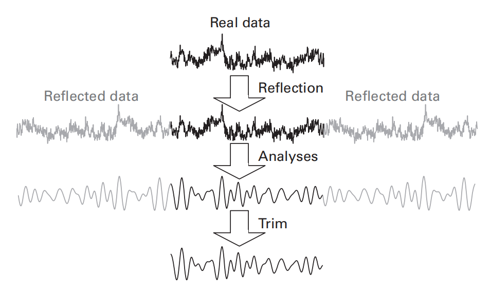
对于时频分析,需要划分更长的时间段,以避免边缘伪影(edge artifacts),即需要预留足够长的缓冲区,使边缘伪影消退。此外,提取的频带越小,需要预留的缓冲区也应该越长。在时频功率谱中,边缘伪影很容易识别,因此可以先试分析一组数据再确定需要预留的缓冲区长度。通常情况下,将缓冲区长度设置为所分析的最低频率所对应的三个周期就足够了(例如,对2Hz的频率,设置缓冲区为1500ms)。
如果划分的epoch不够长,可以使用“reflection”的方法,即将这一段数据关于开始和结尾时刻首尾对称一下,再拼接到数据前和数据后,这样就可以得到三倍长的epoch。
Matching Trial Count across Conditions | Trial数量的设置与平衡
1. 不同的实验条件尽量设置相同的trial数:
理想情况下,所有条件(例如实验设计中的不同实验条件或组别)应该有相同数量的试验。这样可以确保分析结果的公平性和可比性。
2. trial数量对不同分析的影响:
- 基于相位的分析:相位分析对试验数量特别敏感。如果trial数量较少,结果中会出现正偏差(positive bias),即trial数量少的实验条件可能显示出更大的结果。这是因为相位分析对于小样本量更容易受到随机波动的影响,导致条件间结果的偏差。
- 基于功率的分析:功率分析也可能出现一些正偏差。因为功率值通常是正值,数据中的噪声更倾向于增加功率值,所以较少的试验数量可能导致功率结果偏高。
- xxxxxxxxxx % 运行该代码前请先运行Exercise_04_AmatC = NaN(32,3); % 第一、二列为matA的行、列坐标,第三列为该坐标上的元素是否大于0.5countRowi = 1;for rowi = 1:size(matA,1) for coli = 1:size(matA,2) matC(countRowi,1) = rowi; matC(countRowi,2) = coli; if matA(rowi,coli) > 0.5 matC(countRowi,3) = 1; else matC(countRowi,3) = 0; end countRowi = countRowi + 1; endend% 将matC写入txt文件fileC = fopen(‘data_output_04C.txt’,’w’);% variable labelsvariable_labels = {‘row’;’column’;’result’};% 写入第一行变量名for vari=1:length(variable_labels) fprintf(fileC,’%s\t’,variable_labels{vari});end% 换行fprintf(fileC,’\n’);for datarowi=1:size(matC,1) for columni=1:size(matC,2) fprintf(fileC,’%g\t’,matC(datarowi,columni)); end fprintf(fileC,’\n’);endfclose(fileC);matlab
3. 应对低trial数量的方法:
对于ERP分析,如果试验数量较少,与其依赖峰值时间(peak times)的分析,不如取一段时间范围内的平均幅值(mean amplitude)。这种方法对噪声更为稳健,不容易受到个别异常值的影响。
4. 应对不同实验条件的trial数量不一致的方法:
如果出现不同的实验条件下的trial数目不一致,假设最小的trial数为N,那么可以通过以下方法来平衡trial数:
- (不建议采用)直接选前N个trial
- 随机选N个trial
- 根据一些相关的行为或实验变量,如反应时间等,有目的地选N个trial
Trial Rejection
Chapter 9 Overview of Time-Domain EEG Analyses
Event-Related Potentials (ERPs)
To create ERPs, simply align the time-domain EEG to the time=0 event (this was probably already done during preprocessing) and average across trials at each time point.
- 指定 time points
- trial average
Butterfly Plots
A butterfly ploy shows the ERP from all electrodes overlaid in the same figure.
Global Field Power / Topographical Variance Plots
The global field power is the standard deviation of activity over all electrodes.
The Flicker Effect
The flicker effect in EEG research refers to entrainment of brain activity to a rhythmic extrinsic driving factor. This effect is also referred to as steady-state evoked potential, frequency tagging, SSVEP (steady-state visual evoked potential), SSAEP (auditory evoked potential), or something similar.
The flicker effect is arguably an underutilized tool in cognitive electrophysiology. The main benefit of the flicker effect is that it allows you to “ tag ” the processing of a specific stimulus.
(from ChatGPT)
假设你正在进行一项视觉注意力的研究,目的是研究大脑如何同时处理多个视觉刺激。你在屏幕上呈现两个物体:一个物体以12 Hz的频率闪烁(即每秒闪烁12次),另一个物体以15 Hz的频率闪烁。你让参与者专注于两个物体之一,然后使用EEG记录他们的大脑活动。
在这种情况下,闪烁效应会导致大脑中处理视觉信息的区域(通常是视觉皮层)出现与这两个频率相对应的节律性活动。12 Hz的物体会在大脑中产生12 Hz的节律性活动,15 Hz的物体会产生15 Hz的节律性活动。通过分析EEG数据中的频率成分,你可以识别出大脑中对应这两个不同频率的活动区域。
即使EEG无法像功能性磁共振成像(fMRI)那样精确地显示大脑中具体的活动区域,你仍然可以通过这些频率标记来“分离”出大脑中对12 Hz和15 Hz刺激分别作出反应的神经元群体。换句话说,虽然EEG的空间分辨率较低,但通过闪烁效应,你可以“假设”出对不同刺激反应的特定神经区域。
具体的例子说明:
12 Hz闪烁的物体:如果参与者主要关注这个物体,你会看到EEG数据中12 Hz频率的功率增加,这表明视觉皮层中的某个区域在处理这个物体。
15 Hz闪烁的物体:如果参与者关注这个物体,EEG数据中15 Hz频率的功率会增加,显示另一个区域在处理这个物体。
通过这种方法,即使两个物体在大脑中产生的活动区域相距较近,由于频率不同,你依然能够区分开来。这就相当于“模拟”出了一种高空间分辨率,使得你可以推断大脑中不同区域对不同刺激的反应。
Topographical Maps
Creating a topographical map is conceptually similar to interpolating an electrode, except that instead of estimating the activity at one point in space corresponding to a missing electrode, activity is estimated at many point in space between electrodes.
topoplot() |
Microstates
In EEG as well as ERP map series, for brief, subsecond time periods, map landscapes typically remain quasi-stable, then change very quickly into different landscapes.
Durations tend to be around the alpha range (70-130 ms), and topographical distributions tend to fit into four or five distinct patterns.
ERP Images
An ERP image is a 2-D representation of the EEG data from a single electrode. Rather than all trials averaged together to form an ERP, the single-trial EEG traces are stacked vertically and then color coded to show changes in amplitude as changes in color.