Exercises Part 2 | Analyzing Neural Time Series Data
发表于|更新于
|字数总计:490|阅读时长:3分钟|阅读量:
9.8 Exercise
9.8.1
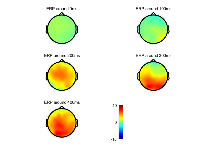
Compute the ERP at each electrode. Select five time points at which to show topographical plots (e.g., 0 to 400 ms in 100-ms steps). In one figure, make a series of topographical plots at these time points. To increase the signal-to-noise ratio, make each plot show the average of activity from 20 ms before until 20 ms after each time point. For example, the topographical plot from 200 ms should show average activity from 180 ms until 220 ms. Indicate the center time point in a title on each subplot.
%% Ex_09 (1)
% load EEG data load sampleEEGdata.mat
% Compute the ERP at each electrode ERP = zeros(EEG.nbchan, EEG.pnts); for electrode_i = 1:EEG.nbchan ERP(electrode_i,:) = squeeze(mean(EEG.data(electrode_i,:,:),3)); end
%% % select 5 time points (0 to 400ms in 100-ms steps) % and plot topographical Maps dt = 20; figure; for timei=0:100:400 % Each point show the average of activity from 20ms before until 20ms % after each point TimeSpani = find(EEG.times >= timei-dt & EEG.times <= timei+dt); MeanEEG = mean(EEG.data(:,TimeSpani,:),2); % topographical plots subplot(3,2,timei/100+1); c = squeeze(mean(MeanEEG(:,:,:),3)); topoplot(double(c),EEG.chanlocs,'plotrad',.53,'electrodes','off','numcontour',0); set(gca,'Clim',[-10,10]); % 统一各subplot的colorbar title(['ERP around ' num2str(timei) 'ms']);
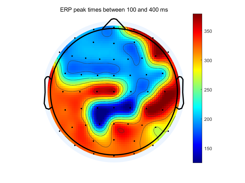
Loop through each electrode and find the peak time of the ERP between 100 and 400 ms. Store these peak times in a separate variable and then make a topographical plot of the peak times (that is, the topographical map will illustrate times in milliseconds, not activity at peak times). Include a color bar in the figure and make sure to show times in milliseconds from time 0 (not, for example, time in milliseconds since 100 ms or indices instead of milliseconds). What areas of the scalp show the earliest and the latest peak responses to the stimulus within this window?
%% Ex_09 (2)

PeakTimes = zeros(EEG.nbchan,1);      % the peak time of the ERP between 100 and 400ms (in ms)
PeakTimedx = zeros(EEG.nbchan,1);      % peak time index of each channel
Timedx = find(EEG.times >= 100 & EEG.times <= 400);     % index of 100~400ms

% find ERP peak times
for electrode_i = 1:EEG.nbchan
    PeakTimedx(electrode_i) = Timedx(1);
    for timespani = 1:length(Timedx)
        if ERP(electrode_i,Timedx(timespani)) > ERP(electrode_i,PeakTimedx(electrode_i))
            PeakTimedx(electrode_i) = Timedx(timespani);
        end
    end
    PeakTimes(electrode_i) = EEG.times(PeakTimedx(electrode_i));
end

% plot a topographical plot of peak times
figure
topoplot(PeakTimes,EEG.chanlocs,'plotrad',.53);
colormap jet
set(gca,'Clim',[min(PeakTimes) max(PeakTimes)]);
colorbar
title('ERP peak times between 100 and 400 ms')